3. Example Analysis with Screenshots
3.a
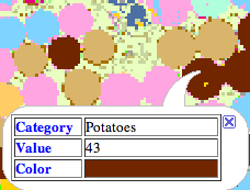
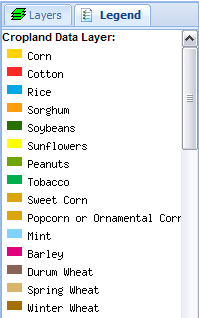
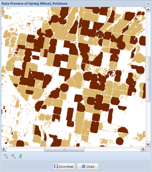
Each pixel within a Cropland Data Layer has a category name, category value, and a defined color. The color and category name are also available within the Legend tab next to the Layer selection.
3.b Define Area of Interest
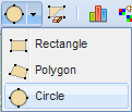
It is necessary to define an Area of Interest (AOI) in order to perform any analysis. There are four ways to select an AOI.
3.b.iBy State/Agricultural Statistics District/County
You can select an AOI by state, by Agricultural Statistics District within a state, or by County within a state. You can only select districts or counties within one state at a time.
The selected area of interest will be highlighted.

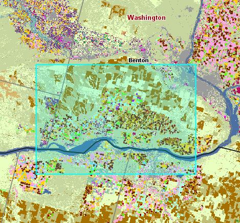
3.b.ii By Rectangle
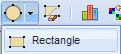
Click and drag to define rectangular AOI
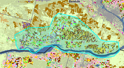
3.b.iii by Polygon
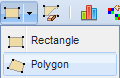
To define a polygon area of interest, click around the boundary of the area. Double click to finish AOI.
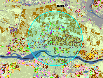
3.b.iv By Circle
Start by clicking in the center of the circle and dragging outward.
3.c Generate Statistics
Once an Area of Interest is selected, click on the Generate Statistics
For a visual representation of the table data click on the Pie Chart
To obtain a map of one or more categories within an Area of Interest click

Use the
3.d
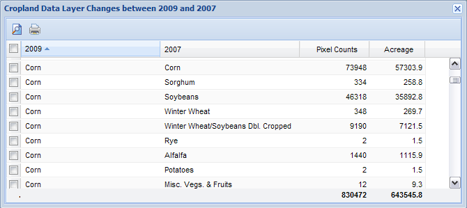
To perform a Change Analysis, select an Area of Interest and two Cropland Data Layers (CDLs) to compare. Once the AOI is selected click the Change Analysis
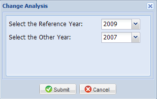
The resulting table will detail how many pixels changed from one category to another between the two selected CDLs. In the change analysis table below 46,318 pixels (35,892.8 acres) of soybeans in 2007 changed to corn in 2009.
3.e.i
If no Area of Interest is selected, clicking the
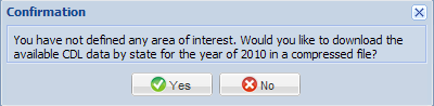
3.e.ii
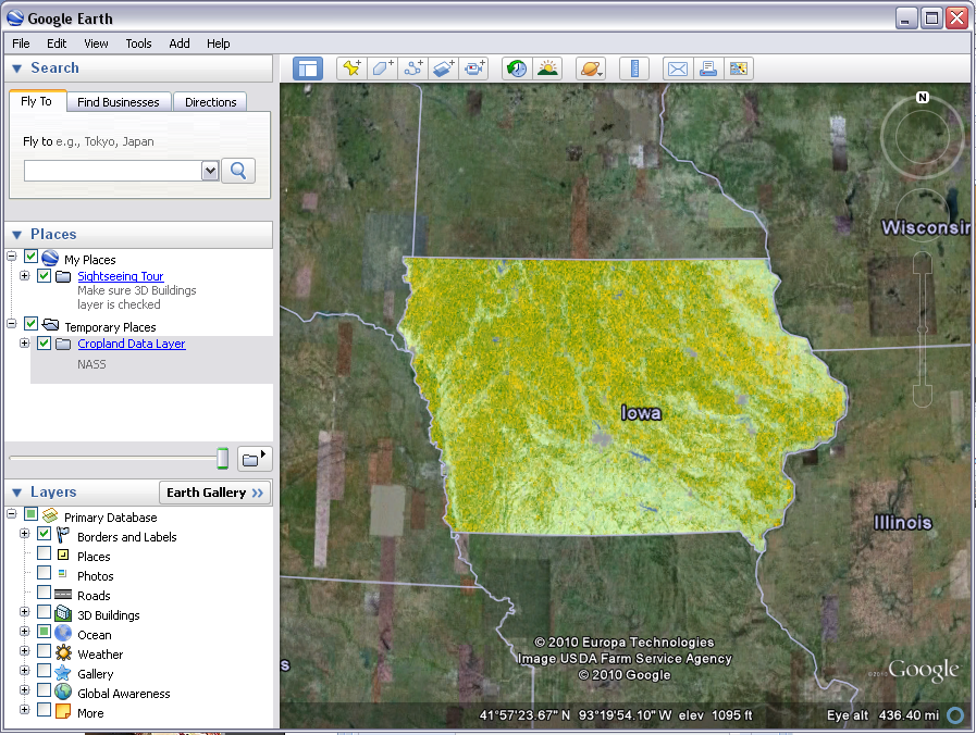
Select an Area of Interest to display in Google Earth. Click on the
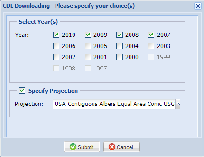
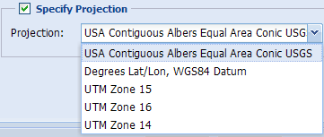
There are multiple projections to choose from. The default projection is USA Contiguous Albers Equal Area Conic USGS. Use the pull down menu to choose which projection is desired.
Click Submit to select Downloading options.
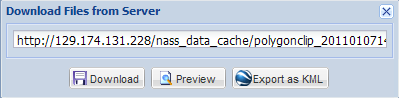
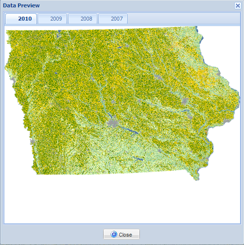
To preview all selected CDLs, click
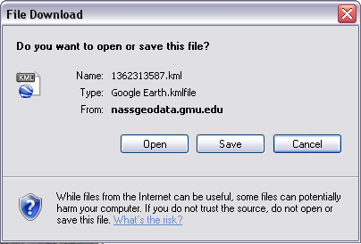
To import into Google Earth, click
If Google Earth is running, select Open to download directly into Google Earth.